Finite Element Analysis (FEA): Pre-processing
The following four-article series was published in a newsletter of the American Society of Mechanical Engineers (ASME). It serves as an introduction to the recent analysis discipline known as the finite element method (FEM). The author is an engineering consultant and expert witness specializing in finite element analysis.
FINITE ELEMENT ANALYSIS: Pre-processing
by Steve Roensch, President, Roensch & Associates
Second in a four-part series
As discussed in Finite Element Analysis (FEA): Introduction, finite element analysis is comprised of pre-processing, solution and post-processing phases. The goals of pre-processing are to develop an appropriate finite element mesh, assign suitable material properties, and apply boundary conditions in the form of restraints and loads.
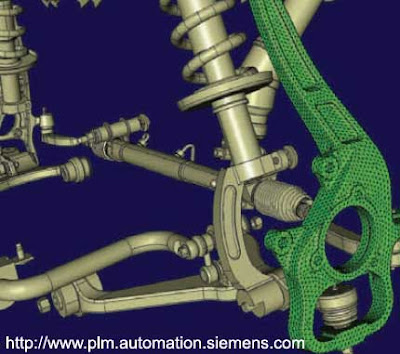 The finite element mesh subdivides the geometry into elements, upon which are found nodes. The nodes, which are really just point locations in space, are generally located at the element corners and perhaps near each midside. For a two-dimensional (2D) analysis, or a three-dimensional (3D) thin shell analysis, the elements are essentially 2D, but may be "warped" slightly to conform to a 3D surface. An example is the thin shell linear quadrilateral; thin shell implies essentially classical shell theory, linear defines the interpolation of mathematical quantities across the element, and quadrilateral describes the geometry. For a 3D solid analysis, the elements have physical thickness in all three dimensions. Common examples include solid linear brick and solid parabolic tetrahedral elements. In addition, there are many special elements, such as axisymmetric elements for situations in which the geometry, material and boundary conditions are all symmetric about an axis.
The model's degrees of freedom (dof) are assigned at the nodes. Solid elements generally have three translational dof per node. Rotations are accomplished through translations of groups of nodes relative to other nodes. Thin shell elements, on the other hand, have six dof per node: three translations and three rotations. The addition of rotational dof allows for evaluation of quantities through the shell, such as bending stresses due to rotation of one node relative to another. Thus, for structures in which classical thin shell theory is a valid approximation, carrying extra dof at each node bypasses the necessity of modeling the physical thickness. The assignment of nodal dof also depends on the class of analysis. For a thermal analysis, for example, only one temperature dof exists at each node.
Developing the mesh is usually the most time-consuming task in FEA. In the past, node locations were keyed in manually to approximate the geometry. The more modern approach is to develop the mesh directly on the CAD geometry, which will be (1) wireframe, with points and curves representing edges, (2) surfaced, with surfaces defining boundaries, or (3) solid, defining where the material is. Solid geometry is preferred, but often a surfacing package can create a complex blend that a solids package will not handle. As far as geometric detail, an underlying rule of FEA is to "model what is there", and yet simplifying assumptions simply must be applied to avoid huge models. Analyst experience is of the essence.
The geometry is meshed with a mapping algorithm or an automatic free-meshing algorithm. The first maps a rectangular grid onto a geometric region, which must therefore have the correct number of sides. Mapped meshes can use the accurate and cheap solid linear brick 3D element, but can be very time-consuming, if not impossible, to apply to complex geometries. Free-meshing automatically subdivides meshing regions into elements, with the advantages of fast meshing, easy mesh-size transitioning (for a denser mesh in regions of large gradient), and adaptive capabilities. Disadvantages include generation of huge models, generation of distorted elements, and, in 3D, the use of the rather expensive solid parabolic tetrahedral element. It is always important to check elemental distortion prior to solution. A badly distorted element will cause a matrix singularity, killing the solution. A less distorted element may solve, but can deliver very poor answers. Acceptable levels of distortion are dependent upon the solver being used.
Material properties required vary with the type of solution. A linear statics analysis, for example, will require an elastic modulus, Poisson's ratio and perhaps a density for each material. Thermal properties are required for a thermal analysis. Examples of restraints are declaring a nodal translation or temperature. Loads include forces, pressures and heat flux. It is preferable to apply boundary conditions to the CAD geometry, with the FEA package transferring them to the underlying model, to allow for simpler application of adaptive and optimization algorithms. It is worth noting that the largest error in the entire process is often in the boundary conditions. Running multiple cases as a sensitivity analysis may be required.
FINITE ELEMENT ANALYSIS: Pre-processing
by Steve Roensch, President, Roensch & Associates
Second in a four-part series
As discussed in Finite Element Analysis (FEA): Introduction, finite element analysis is comprised of pre-processing, solution and post-processing phases. The goals of pre-processing are to develop an appropriate finite element mesh, assign suitable material properties, and apply boundary conditions in the form of restraints and loads.
The finite element mesh subdivides the geometry into elements, upon which are found nodes. The nodes, which are really just point locations in space, are generally located at the element corners and perhaps near each midside. For a two-dimensional (2D) analysis, or a three-dimensional (3D) thin shell analysis, the elements are essentially 2D, but may be "warped" slightly to conform to a 3D surface. An example is the thin shell linear quadrilateral; thin shell implies essentially classical shell theory, linear defines the interpolation of mathematical quantities across the element, and quadrilateral describes the geometry. For a 3D solid analysis, the elements have physical thickness in all three dimensions. Common examples include solid linear brick and solid parabolic tetrahedral elements. In addition, there are many special elements, such as axisymmetric elements for situations in which the geometry, material and boundary conditions are all symmetric about an axis.The model's degrees of freedom (dof) are assigned at the nodes. Solid elements generally have three translational dof per node. Rotations are accomplished through translations of groups of nodes relative to other nodes. Thin shell elements, on the other hand, have six dof per node: three translations and three rotations. The addition of rotational dof allows for evaluation of quantities through the shell, such as bending stresses due to rotation of one node relative to another. Thus, for structures in which classical thin shell theory is a valid approximation, carrying extra dof at each node bypasses the necessity of modeling the physical thickness. The assignment of nodal dof also depends on the class of analysis. For a thermal analysis, for example, only one temperature dof exists at each node.
Developing the mesh is usually the most time-consuming task in FEA. In the past, node locations were keyed in manually to approximate the geometry. The more modern approach is to develop the mesh directly on the CAD geometry, which will be (1) wireframe, with points and curves representing edges, (2) surfaced, with surfaces defining boundaries, or (3) solid, defining where the material is. Solid geometry is preferred, but often a surfacing package can create a complex blend that a solids package will not handle. As far as geometric detail, an underlying rule of FEA is to "model what is there", and yet simplifying assumptions simply must be applied to avoid huge models. Analyst experience is of the essence.
The geometry is meshed with a mapping algorithm or an automatic free-meshing algorithm. The first maps a rectangular grid onto a geometric region, which must therefore have the correct number of sides. Mapped meshes can use the accurate and cheap solid linear brick 3D element, but can be very time-consuming, if not impossible, to apply to complex geometries. Free-meshing automatically subdivides meshing regions into elements, with the advantages of fast meshing, easy mesh-size transitioning (for a denser mesh in regions of large gradient), and adaptive capabilities. Disadvantages include generation of huge models, generation of distorted elements, and, in 3D, the use of the rather expensive solid parabolic tetrahedral element. It is always important to check elemental distortion prior to solution. A badly distorted element will cause a matrix singularity, killing the solution. A less distorted element may solve, but can deliver very poor answers. Acceptable levels of distortion are dependent upon the solver being used.
Material properties required vary with the type of solution. A linear statics analysis, for example, will require an elastic modulus, Poisson's ratio and perhaps a density for each material. Thermal properties are required for a thermal analysis. Examples of restraints are declaring a nodal translation or temperature. Loads include forces, pressures and heat flux. It is preferable to apply boundary conditions to the CAD geometry, with the FEA package transferring them to the underlying model, to allow for simpler application of adaptive and optimization algorithms. It is worth noting that the largest error in the entire process is often in the boundary conditions. Running multiple cases as a sensitivity analysis may be required.

Comments